31: Confidence Intervals (Concept)

Source: Statistical Inference via Data Science: A Modern Dive into R and the Tidyverse
Chapter 8: Bootstrapping and Confidence Intervals
https://moderndive.com/8-confidence-intervals.html

Setting: Pennies

Among pennies in circulation in 2019, what was the average year of minting? We have a sample size of 50 pennies.

# looking at the data set
pennies_sample

# A tibble: 50 × 2
      ID  year
   <int> <dbl>
 1     1  2002
 2     2  1986
 3     3  2017
 4     4  1988
 5     5  2008
 6     6  1983
 7     7  2008
 8     8  1996
 9     9  2004
10    10  2000
# ℹ 40 more rows

Sample Distribution

# visualizing the the pennies
pennies_sample %>%
  ggplot(aes(x = year)) +
  geom_dotplot(binwidth = 1, color = "tan3", fill = "tan4") +
  labs(title = "Pennies Sample",
       subtitle = "observed in 2019",
       caption = "Source: Modern Dive",
       x = "year",
       y = "proportion")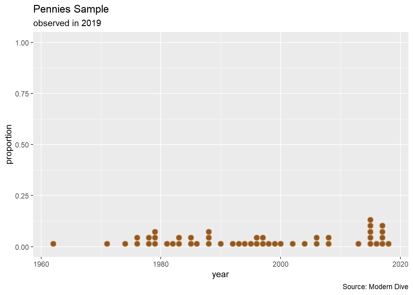

# visualizing the distribution of the pennies
p1 <- pennies_sample %>%
  ggplot(aes(x = year)) +
  geom_histogram(binwidth = 10, color = "tan3", fill = "tan4") +
  labs(title = "Pennies Sample",
       subtitle = "observed in 2019",
       caption = "Source: Modern Dive")

# display graph (in addition to storing the graph in a variable)
p1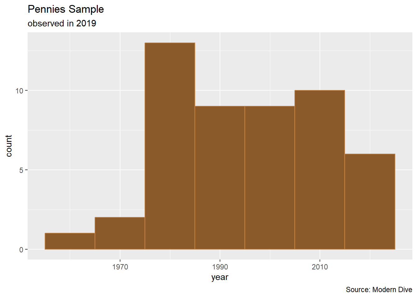

# sample mean
pennies_sample %>% summarize(xbar = mean(year))

# A tibble: 1 × 1
   xbar
  <dbl>
1 1995.

Resampling

Using the available sample of data to fabricate another sample is called resampling.

Resampling Once

Suppose that we took the 50 pennies and resampled once while sampling with replacement.

pennies_resampled_once <- pennies_sample %>%
  sample_n(size = 50, replace = TRUE)

# visualizing the distribution of the pennies
p2 <- pennies_resampled_once %>%
  ggplot(aes(x = year)) +
  geom_histogram(binwidth = 10, color = "tan3", fill = "tan4") +
  labs(title = "Pennies Resampled Once",
       subtitle = "sampled with replacement",
       caption = "Source: Modern Dive")

# (using `patchwork` package to arrange plots side-by-side
p1 + p2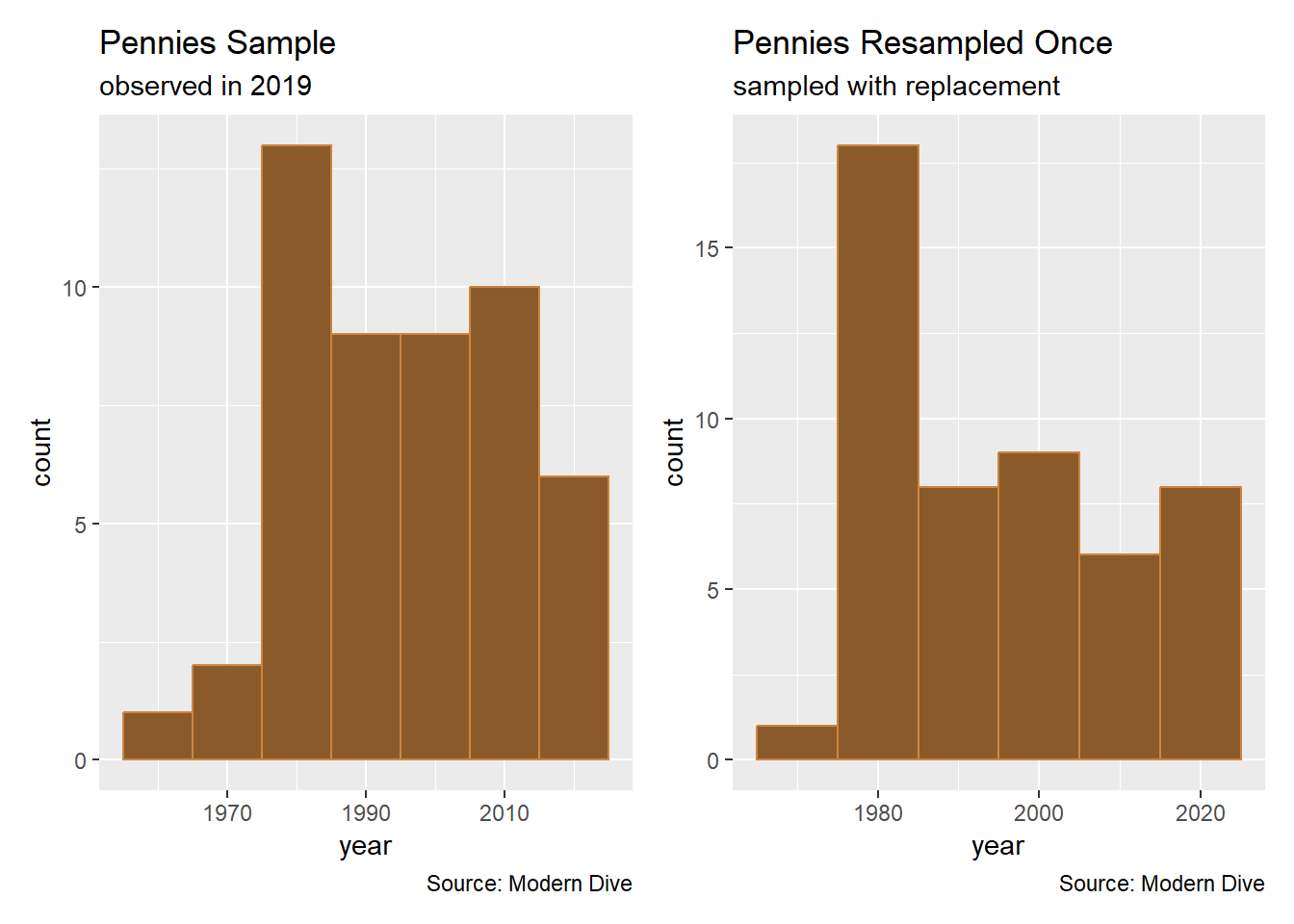

# a different sample mean
pennies_resampled_once %>% summarize(xbar = mean(year))

# A tibble: 1 × 1
   xbar
  <dbl>
1 1995.

Resampled Many Times

Suppose now that we have each person in a 30-student discussion section repeat the act of drawing those 50 pennies with replacement.

pennies_resampled_many <- pennies_sample %>%
  rep_sample_n(size = 50, replace = TRUE, reps = 30)

Now we have each virtual student report their mean year.

pennies_resampled_many %>%
  group_by(replicate) %>%
  summarize(mean_year = mean(year))

# A tibble: 30 × 2
   replicate mean_year
       <int>     <dbl>
 1         1     1998.
 2         2     1991.
 3         3     1996.
 4         4     1991.
 5         5     1998.
 6         6     1995.
 7         7     1993.
 8         8     1994.
 9         9     1997.
10        10     1995.
# ℹ 20 more rows

summary(pennies_sample$year)

   Min. 1st Qu.  Median    Mean 3rd Qu.    Max. 
   1962    1983    1996    1995    2008    2018

pennies_resampled_many %>%
  group_by(replicate) %>%
  mutate(mean_year = mean(year)) %>%
  ungroup() %>%
  select(replicate, mean_year) %>%
  distinct() %>%
  ggplot(aes(x = mean_year)) +
  geom_histogram(binwidth = 1, color = "tan3", fill = "tan4") +
  labs(title = "Resampling Results",
       subtitle = "N = 30 resamples",
       caption = "Source: Modern Dive")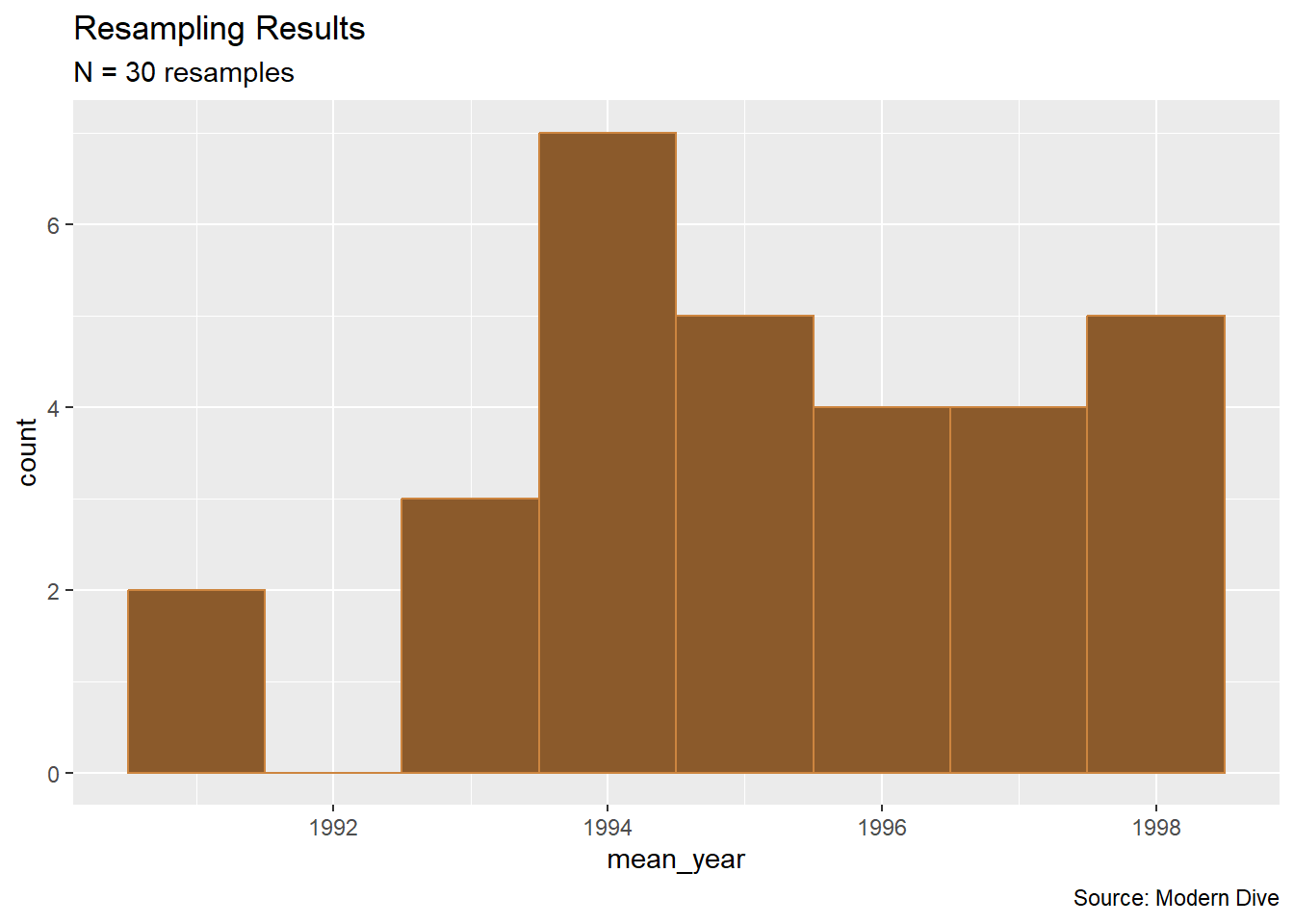

Out of curiosity, let us push this process to \(N = 1337\) resamples.

pennies_resampled_means <- pennies_sample %>%
  rep_sample_n(size = 50, replace = TRUE, reps = 1337) %>%
  group_by(replicate) %>%
  mutate(mean_year = mean(year)) %>%
  ungroup() %>%
  select(replicate, mean_year) %>%
  distinct() 

pennies_resampled_means %>%
  ggplot(aes(x = mean_year)) +
  geom_histogram(binwidth = 1, color = "tan3", fill = "tan4") +
  labs(title = "Resampling Results",
       subtitle = "N = 1337 resamples",
       caption = "Source: Modern Dive")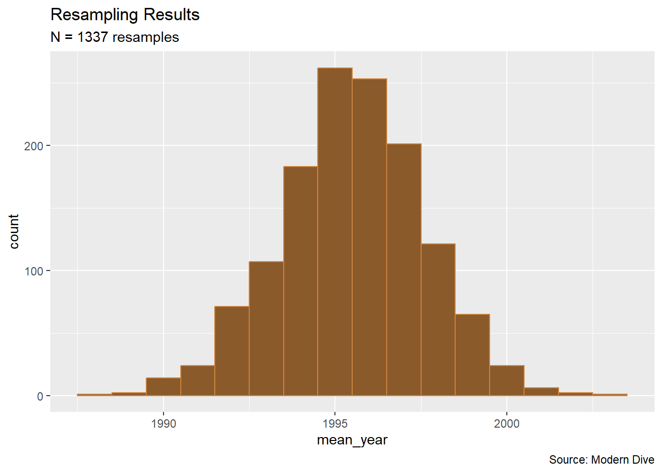

Confidence Intervals

Toward Confidence Intervals

The standard deviation of a sampling distribution is called the standard error.

xbar <- mean(pennies_resampled_means$mean_year)
SE   <- sd(pennies_resampled_means$mean_year)

We can build a 95% confidence interval by computing \(\bar{x} \pm 1.96*SE\)

c(xbar - 1.96*SE, xbar + 1.96*SE)

[1] 1991.377 1999.624

pennies_resampled_means %>%
  ggplot(aes(x = mean_year)) +
  geom_histogram(binwidth = 1, color = "tan3", fill = "tan4") +
  geom_vline(xintercept = c(xbar - 1.96*SE, xbar + 1.96*SE), color = "yellow", linewidth = 2) +
  labs(title = "Resampling Results",
       subtitle = "N = 1337 resamples",
       caption = "Source: Modern Dive") +
  theme_minimal()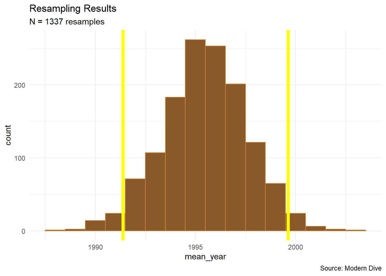

Using the infer package

pennies_sample %>%
  specify(response = year)

Response: year (numeric)
# A tibble: 50 × 1
    year
   <dbl>
 1  2002
 2  1986
 3  2017
 4  1988
 5  2008
 6  1983
 7  2008
 8  1996
 9  2004
10  2000
# ℹ 40 more rows

pennies_sample %>%
  specify(response = year) %>%
  calculate(stat = "mean")

Response: year (numeric)
# A tibble: 1 × 1
   stat
  <dbl>
1 1995.

pennies_sample %>%
  specify(response = year) %>%
  generate(reps = 1337, type = "bootstrap")

Response: year (numeric)
# A tibble: 66,850 × 2
# Groups:   replicate [1,337]
   replicate  year
       <int> <dbl>
 1         1  1983
 2         1  1992
 3         1  2015
 4         1  2018
 5         1  1997
 6         1  1988
 7         1  2017
 8         1  1976
 9         1  1985
10         1  2015
# ℹ 66,840 more rows

bootstrap_distribution <- pennies_sample %>%
  specify(response = year) %>%
  generate(reps = 1337, type = "bootstrap") %>%
  calculate(stat = "mean")

# print
bootstrap_distribution

Response: year (numeric)
# A tibble: 1,337 × 2
   replicate  stat
       <int> <dbl>
 1         1 1998.
 2         2 1994.
 3         3 1990.
 4         4 1998.
 5         5 1996.
 6         6 1996.
 7         7 1998.
 8         8 1996.
 9         9 1998.
10        10 1993.
# ℹ 1,327 more rows

Bootstrap Distribution

The resulting distribution from sampling without replacement is called a bootstrap distribution

visualise(bootstrap_distribution)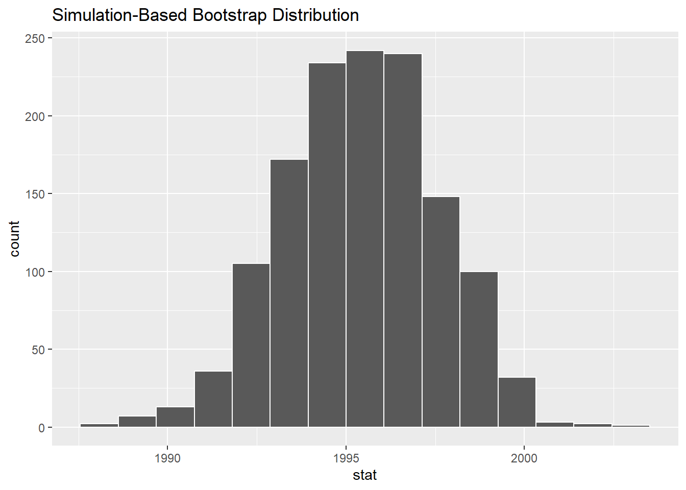

Infer get_ci()

There are also wrappers in the infer package to extract the confidence interval

bootstrap_distribution %>%
  get_confidence_interval(point_estimate = mean(bootstrap_distribution$stat), 
                          level = 0.95, type = "se")

# A tibble: 1 × 2
  lower_ci upper_ci
     <dbl>    <dbl>
1    1991.    2000.

Alternatively, we can use percentiles to build our confidence intervals. This is useful when the data is not normally distributed.

bootstrap_distribution %>%
  get_confidence_interval(level = 0.95, type = "percentile")

# A tibble: 1 × 2
  lower_ci upper_ci
     <dbl>    <dbl>
1    1991.    1999.

SE_CI <- bootstrap_distribution %>%
  get_ci(point_estimate = mean(bootstrap_distribution$stat),
         level = 0.95, type = "se")

visualize(bootstrap_distribution) +
  shade_ci(endpoints = SE_CI, color = "#DAA900", fill = "#002856")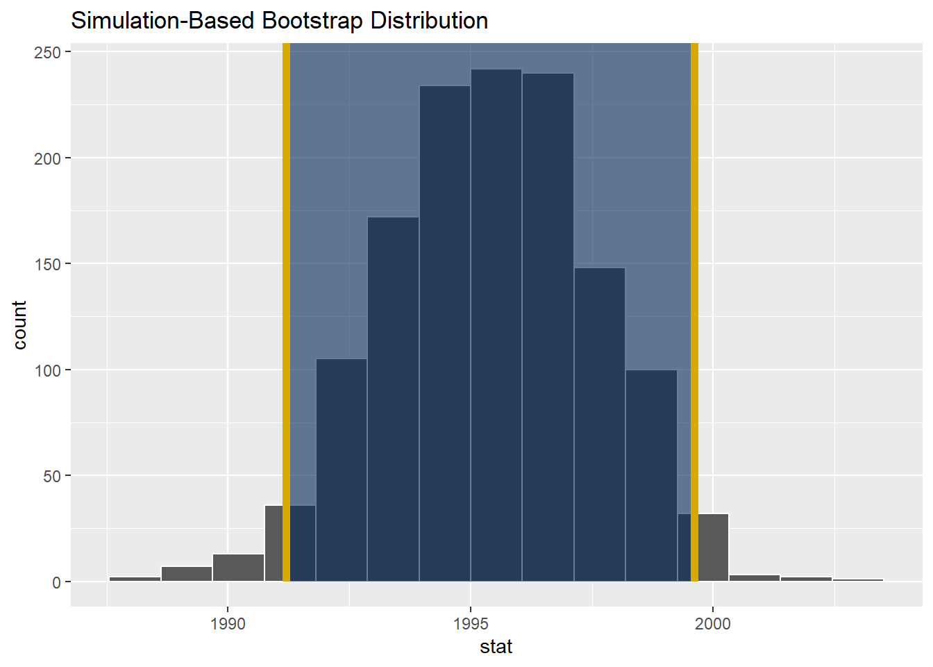

Inference

How do we describe confidence intervals?

Example: Bowl of Marbles

The bowl data was literally a classroom bowl of red and white marbles

bowl %>%
  ggplot(aes(x = color, fill = color)) +
  geom_bar(stat = "count", color = "black") +
  scale_fill_manual(values = c("red", "white")) +
  labs(title = "Bowl of Marbles",
       subtitle = "population is known",
       caption = "Source: Modern Dive")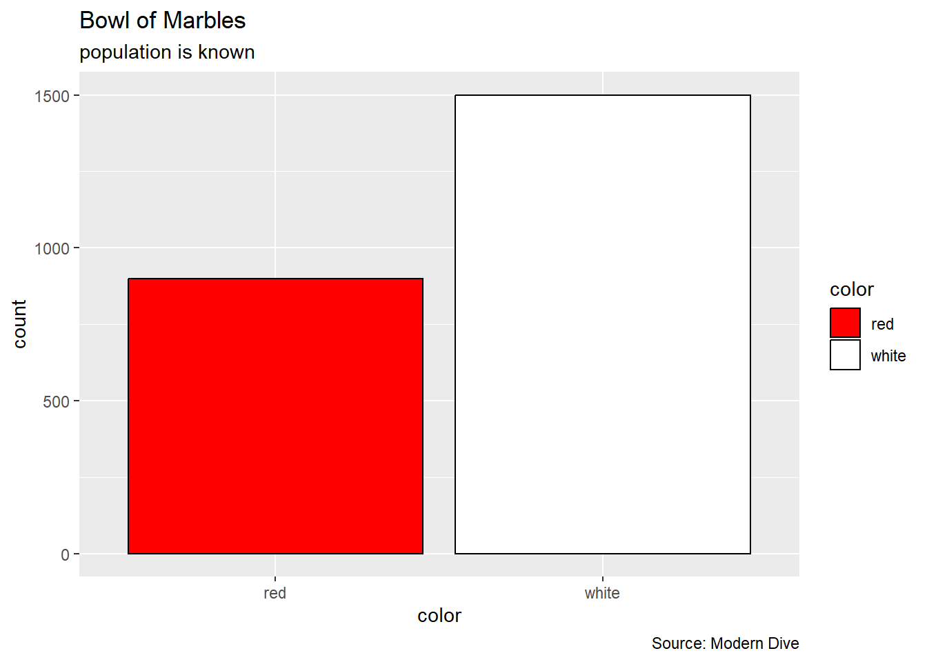

where we know the true proportion of red marbles.

bowl %>%
  summarize(proportion_red = mean(color == "red"))

# A tibble: 1 × 1
  proportion_red
           <dbl>
1          0.375

Simulations

CI_simulation <- function(confidence = 95, sample_size = 25, num_intervals = 10){
  # Constants
  alpha <- 1 - confidence/100
  n <- sample_size
  N <- num_intervals
  proportion_red <- 0.375 #true population proportion
  
  # vector allocation
  left <- rep(NA, N)
  right <- rep(NA, N)
  captured <- rep(NA, N)
  
  for(i in 1:N){
    this_sample <- sample(bowl$color, n, replace = TRUE)
    phat <- mean(this_sample == "red") #sample proportion
    
    #margin of error
    E <- qnorm(1 - alpha/2)*sqrt( phat*(1-phat)/n)
    
    #this confidence interval
    left[i] <- phat - E
    right[i] <- phat + E
    
    #did the confidence interval capture the true proportion?
    captured[i] <- ifelse(left[i] <= proportion_red & right[i] >= proportion_red, TRUE, FALSE)
  }
  
  # graph
  df <- data.frame(left, right, captured)
  ggplot(df, aes(x = left, y = 1:N)) +
    geom_vline(xintercept = proportion_red, color = "black") +
    geom_segment(aes(x = left, y = 1:N, 
                     xend = right, yend = 1:N,
                     color = captured)) +
    labs(title = "Simulation of bowl samples",
         subtitle = paste0("alpha = ", alpha, ", n = ", n),
         caption = "Bio 175", 
         x = "proportion red",
         y = "iteration") +
    theme_minimal()
}

CI_simulation(confidence = 95, sample_size = 25, num_intervals = 100)

Significance Levels
Sample Sizes

p1 <- CI_simulation(80, 25, 100) + theme(legend.position = "none")
p2 <- CI_simulation(95, 25, 100) + theme(legend.position = "none")
p3 <- CI_simulation(99, 25, 100) + theme(legend.position = "none")

p1 + p2 + p3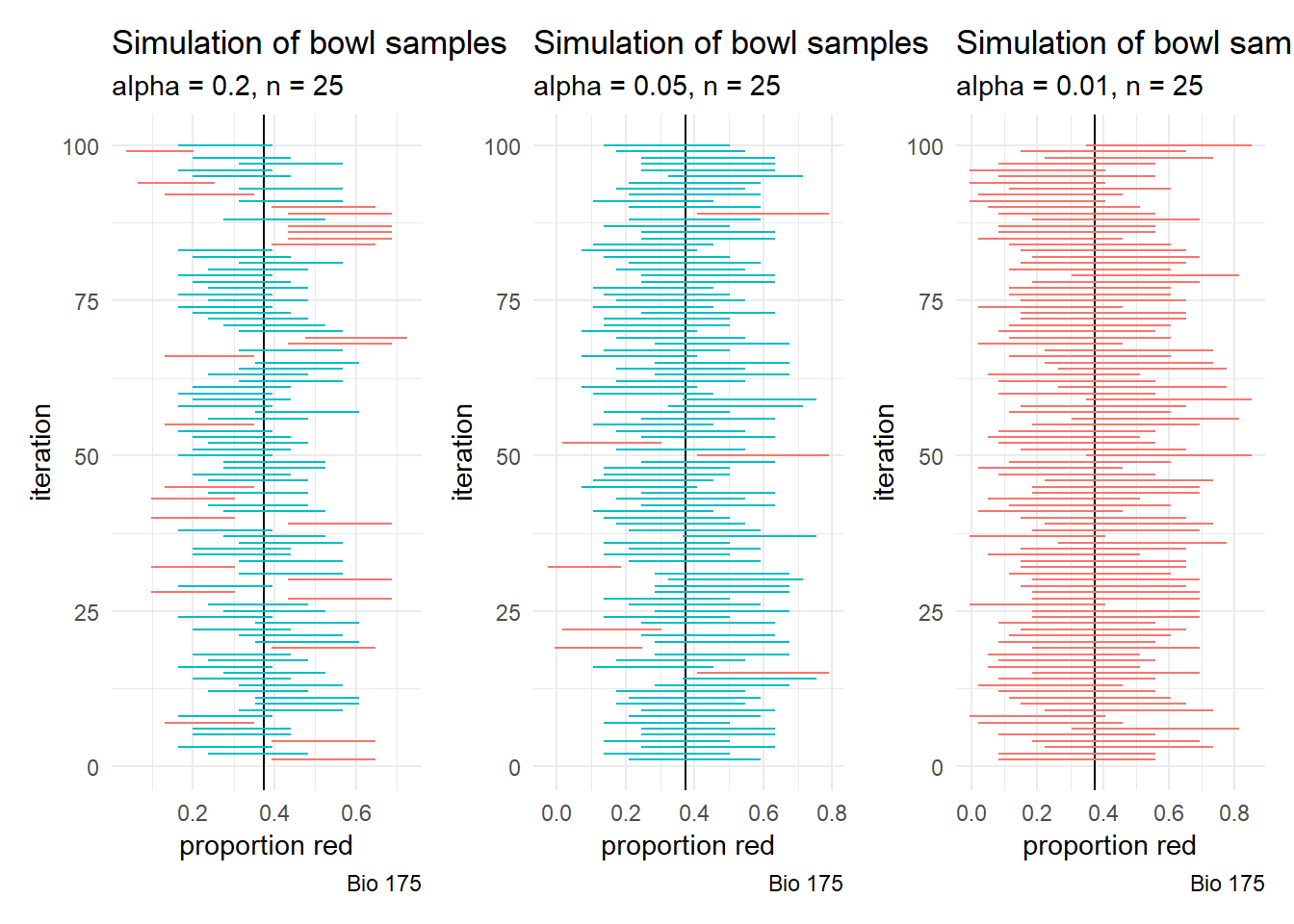

As we request more confidence, the confidence intervals are more likely to include the true population parameter.

p4 <- CI_simulation(95, 25, 100) + theme(legend.position = "none")
p5 <- CI_simulation(95, 100, 100) + theme(legend.position = "none")
p6 <- CI_simulation(95, 400, 100) + theme(legend.position = "none")

p4 + p5 + p6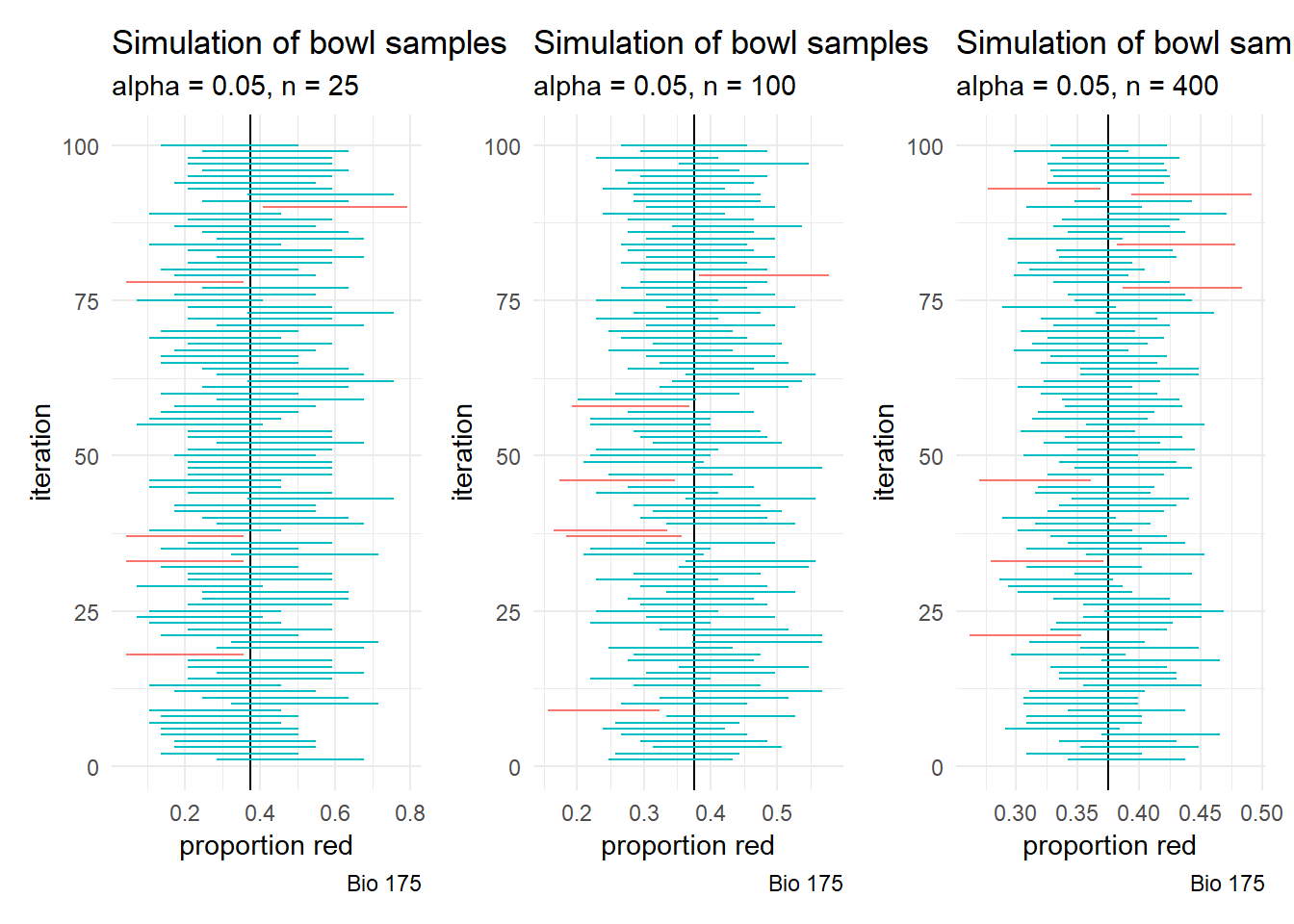

As we use larger sample sizes, the confidence intervals are more likely to include the true population parameter.

Looking Ahead

WHW10 (due today)
WHW11
LHW9
LHW10

Final Exam will be on May 6

more information in weekly announcement

tweet source